Spring 2026 | AE426HON - Spacecraft Attitude Dynamics

Dynamics and Stability of Spacecraft Attitude Systems

MATLAB Rigid Body Dynamics Kinematics ODE Solvers

The Objective

To computationally model and analyze the stability of complex rotational systems. The project was divided into two core phases: verifying the stability of the principal axes for a torque-free rigid body under small perturbations (ε << 1), and modeling the precession, nutation, and spin of a heavy top using Euler angle kinematics.

The Execution

I developed a comprehensive MATLAB simulation framework to solve the exact equations of motion. For the torque-free rigid body, the script simulated both exact equilibrium and perturbed trajectories across the major, minor, and intermediate axes. To ensure physical realism, I implemented a validation layer that continuously calculated Kinetic Energy (T) and Angular Momentum magnitude squared (||H||2), proving conservation laws were maintained throughout the integration.

Implementation Highlight: Custom ODE Constraints

For the spinning top simulation, the physical constraints dictated that the integration should stop if the top "fell" past a certain angle. Rather than running a blind simulation and trimming the data afterward, I integrated a custom event-tracking function directly into MATLAB's ode45 solver to halt execution the exact millisecond the nutation angle (θ) reached 95 degrees.

top_simulation.m

% Configure ODE solver to listen for the nutation limit event
options_part2 = odeset('RelTol', 1e-8, 'AbsTol', 1e-8, 'Events', @nutation_event);
[t2, X] = ode45(@(t,X) top_dynamics(t, X, It, Ia, mgl), tspan_part2, X0, options_part2);

% ... [Dynamics function omitted for brevity] ...

% Custom event function to halt integration at 95 degrees
function [value, isterminal, direction] = nutation_event(~, X)
    target_theta = deg2rad(95);   % Target limit in radians
    theta = X(2);                 % Current nutation angle
    
    value = theta - target_theta; % Zero-crossing triggers the event
    isterminal = 1;               % 1 = Stop the integration
    direction = 0;                % Detect all zero-crossings
end
        

The Result

The simulation successfully mapped the stability profiles of all three principal axes and accurately modeled the non-linear nutation of the heavy top. By explicitly separating handwritten physics logic from AI-assisted data visualization routines, the project maintained absolute academic integrity while delivering highly polished, professional-grade telemetry plots.

View Full Technical Report (PDF) →
Spring 2026 | AE314/315 - Wind Tunnel Lab

Experimental Analysis of a Turbulent Boundary Layer

MATLAB Fluid Mechanics Signal Processing (FFT) Data Reduction

The Objective

To process raw experimental wind tunnel data to characterize a boundary layer, calculate aerodynamic friction coefficients, and determine the largest turbulent eddy frequency using spectral analysis techniques.

The Execution

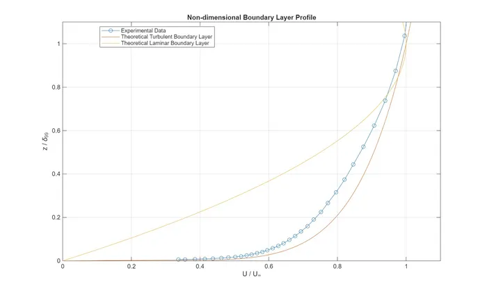
This project required writing a robust data reduction architecture to handle experimental telemetry collected via hot-wire anemometry and pressure transducers. The MATLAB script applied calibration coefficients, tared the sensors, and calculated macroscopic boundary layer metrics like the 99% boundary layer thickness (δ99) and wall shear stress using Sutherland's Law. The velocity profile was then non-dimensionalized to successfully prove it matched the 1/7 theoretical approximation for turbulent flow.

Dimensional Boundary Layer Velocity Profile
Velocity profile matching the 1/7 turbulent approximation.

Implementation Highlight: Spectral Analysis & Welch's Method

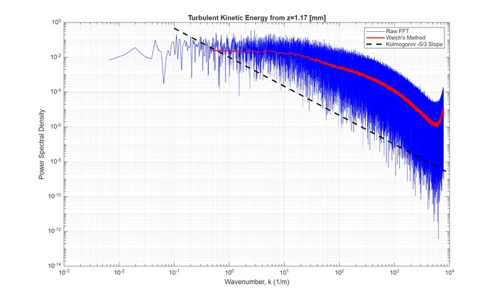
To analyze the microscopic turbulent structures, I applied a Fast Fourier Transform (FFT) to the fluctuating velocity components. Because raw FFT data is notoriously noisy, I implemented Welch's method to compute a smoothed Power Spectral Density (PSD). By plotting this against the wavenumber, I was able to successfully validate the turbulent kinetic energy cascade against the theoretical Kolmogorov -5/3 slope.

Power Spectral Density vs Wavenumber
Power Spectral Density plot validating the Kolmogorov -5/3 turbulent energy cascade.
boundary_layer_fft.m

% Calculate wavenumber (k) using sliced frequencies
k = (2*pi*freqs_sliced) / mean(V_tran);

% Implement Welch's Method for PSD smoothing
segment_length = 2^15;
window = hamming(segment_length);
noverlap = round(segment_length/2);
nfft = segment_length;

[PSD_Welch, f_Welch] = pwelch(V_AC, window, noverlap, nfft, Fs);
k_Welch = (2*pi*f_Welch) / mean(V_tran);

% Isolate largest turbulent eddy frequency
[~, max_idx] = max(PSD_Welch(2:end));
largest_eddy_freq = f_Welch(max_idx + 1);
        

The Result

The code successfully characterized the flow, calculating a free stream velocity of 15.07 m/s, a skin friction coefficient of 0.0027, and isolating the largest turbulent eddy frequency at 6.10 Hz. The data reduction pipeline proved that the experimental wind tunnel data definitively matched theoretical turbulent flow models.

View Full Published Code (PDF) →